I have been asked a couple of times about the use of rotations in Principal Component Analysis (PCA). Each time it is far enough apart that I forget what I said the previous time, so I have written down what I should say here.
What happens in a PCA
Conceptually, PCA commonly is to summarise the latent variation within a dataset. That is, when we want to measure something that is not directly accessible, a way around that is to ask a number of questions that are measurable and combine them in a way that reflects the underlying thing we do want to measure.
A PCA aims to do this mathematically by measuring the correlation between all pairs of variables1, then creating new variables based on those correlations and weights of the original variables through an approach called eigenvalue decomposition. Variables that are similar weight heavily onto the same principal component, and there can be as many principal components as there are variables.
PCA extracts components; rotations such as varimax are post-hoc steps applied after extraction. Varimax is an orthogonal rotation that seeks to simplify loadings by making large weights larger and small weights smaller while keeping components orthogonal (uncorrelated). This combination prioritizes a simpler structure of the principal components.
In most social sciences, assuming that latent variables are uncorrelated is usually a poor assumption. Most aspects of human behaviour impact each other in some way, and so we often want to relax this assumption, using alternative rotations, such as Promax (PROjection to MAXimise simplicity) and ObliMin (OBLIque MINimum). But, often we do not have a good understanding of how these approaches vary or differ in their approach to measuring latent variables. Let us look at this in a simulated example.
In the simulated example, I start with the end product (two latent factors named F1 and F2), then create four variables from these latent factors (V1, V2, V3, V4). F1 and F2 have a 0.2 correlation that I have imposed, which is a low but not negligible relationship between latent variables. This is created below with the code: F2 <- 0.2 * F1 + sqrt(1 - 0.2^2) * rnorm(n), which constructs F2 with approximate correlation 0.2 to F1. I specify the weights so that V1 and V2 are weighted towards F1 (0.8 and 0.7 respectively), and V3 and V4 are weighted towards F2 (0.8; 0.7), and add some normally distributed noise to those variables. The variables V1-V4 then sit in a data frame df. The correlation matrix between each variable shows us that there is a stronger relationship between V1-2 and V3-4 but there is also some relationship across this divided, which is not an uncommon finding in social datasets.
library(psych)library(ggplot2)library(ggpubr)library(GGally)# --- Step 1: Create example data with clear 2-factor structure ---set.seed(123)n <-200F1 <-rnorm(n)F2 <- F1 *0.2+sqrt(1-0.2^2) *rnorm(n)# Variables mainly loading on one factorV1 <-0.8*F1 +0.1*F2 +rnorm(n, 0, 0.2)V2 <-0.7*F1 +0.2*F2 +rnorm(n, 0, 0.2)V3 <-0.1*F1 +0.8*F2 +rnorm(n, 0, 0.2)V4 <-0.2*F1 +0.7*F2 +rnorm(n, 0, 0.2)df <-data.frame(V1, V2, V3, V4)cat("Correlations of Variables:\n")
As mentioned in the description, PCA is based off of a correlation matrix, which is created below in the object R, but you can also put the data frame directly into the function principal. Doing the latter means you will be returned values for each observation in the data frame that reflect the principal components (which is usually what researchers are after).
Loadings:
   RC2   RC1
V1 0.178 0.969
V2 0.348 0.918
V3 0.970 0.168
V4 0.920 0.339

                 RC2   RC1
SS loadings    1.941 1.924
Proportion Var 0.485 0.481
Cumulative Var 0.485 0.966
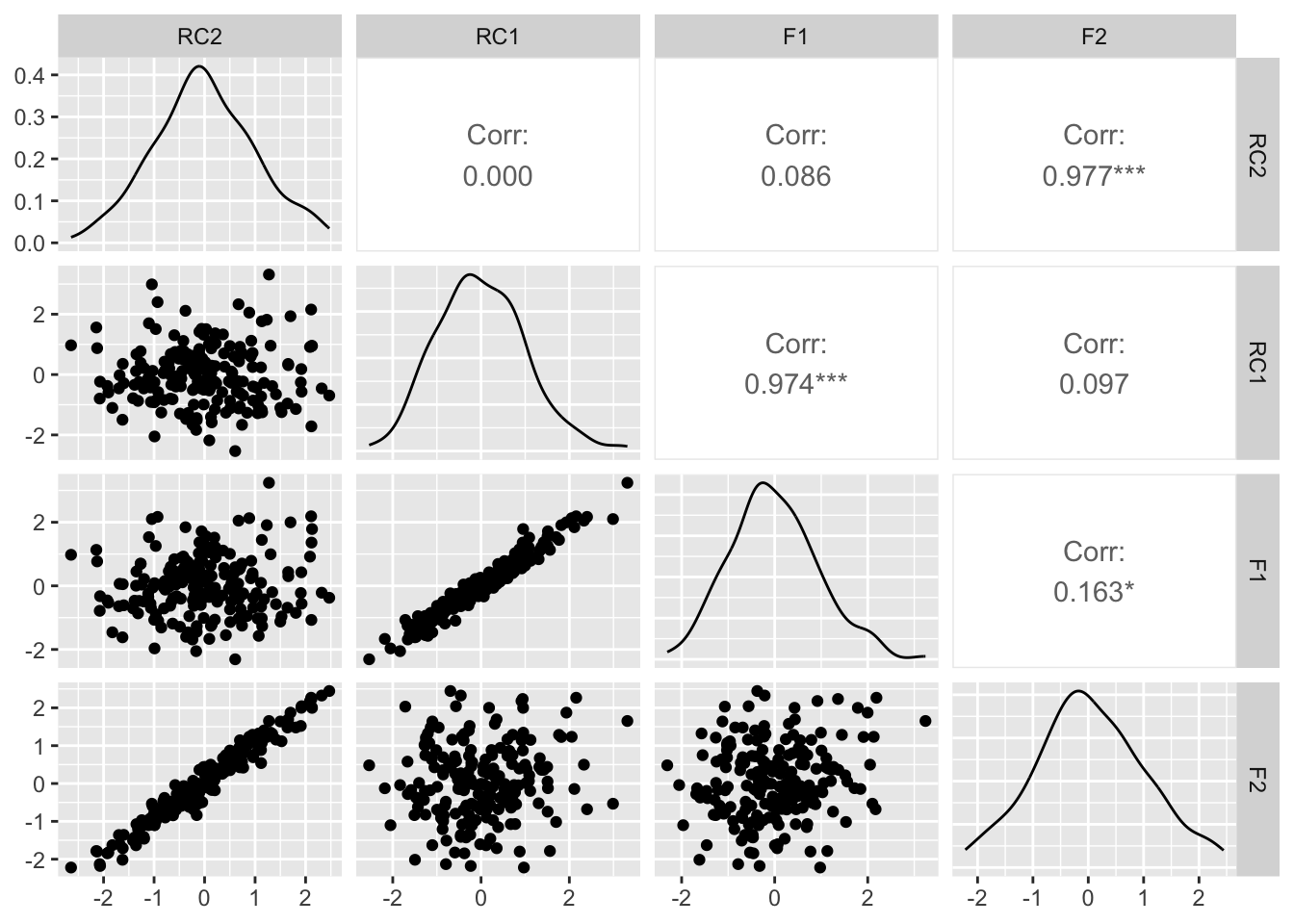
plot_df =data.frame(pc_varimax$scores, F1 , F2)ggpairs(plot_df)
Looking at the loadings for the variables on the principal components the loadings are matching up about as well as we could hope. V1 and V2 load heavily onto RC1 (RC = rotated component) and V3 and V4 on RC2. It does not capture the relationship between the latent variables however, showing a correlation of 0 for RC1 and RC2, which is a consequence of the orthogonality constraint in varimax rotations. What we can be sure of in this approach is that the principal components are independent latent variables, however, in social and human behavioral research, it is more often that latent factors are related in some way - both conceptually and numerically.
As such, we can use different rotations that make adjustments to PCA that relax the orthogonality assumption in order to get more interpretable factors. Two common alternative rotations to varimax used in social research is the ProMax and ObliMin rotations.
ProMax
Promax is an extension of the varimax rotation, that begins with the varimax output and raises the loadings to a power (in addition to the square-square change performed by varimax) . By raising the loadings to a power, the strong loadings become larger and the weak loadings get closer to zero. The effect of this change is that each variable weights more strongly onto each latent variable, and exaggerates the patterns seen in the latent variable. This more significant change to the loadings also makes the latent components correlated, unlike varimax components.
Loadings:
   RC1    RC2
V1  1.028 -0.092
V2  0.922  0.111
V3 -0.094  1.028
V4  0.111  0.921

                 RC1   RC2
SS loadings    1.926 1.925
Proportion Var 0.482 0.481
Cumulative Var 0.482 0.963
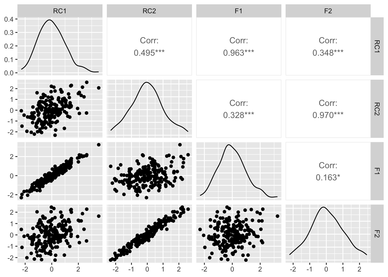
plot_df =data.frame(pc_promax$scores, F1 , F2)ggpairs(plot_df)
The exaggeration of weightings performed by the ProMax rotation further emphasises the weighting between principal components, V1-2 are heavily weighted to RC1 and V3-4 onto RC2, as we expect. However, instead of constraining the correlation between latent variables to zero, the Promax approach has over estimated the latent variation between F1 and F2, with a correlation of 0.533 - more than double the size of the correlation that we imposed between the latent factors.
ObliMin
ObliMin is an oblique rotation (i.e. it relaxes the orthogonality constraint) that directly searches for a simpler loading pattern while allowing factors to correlate. Unlike Promax, which starts from an orthogonal solution and then rotates toward a target, ObliMin directly optimizes a simplicity criterion. In plain terms, that criterion penalizes variables having substantial loadings on more than one factor, so solutions where each variable loads primarily on one factor are favored.
Loadings:
   TC1    TC2
V1  1.018 -0.075
V2  0.917  0.125
V3 -0.076  1.018
V4  0.126  0.915

                 TC1   TC2
SS loadings    1.899 1.895
Proportion Var 0.475 0.474
Cumulative Var 0.475 0.948
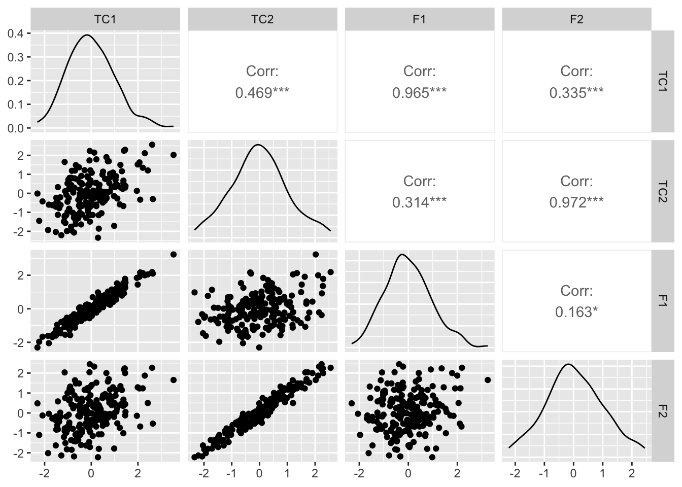
plot_df =data.frame(pc_oblimin$scores, F1 , F2)ggpairs(plot_df)
The ObliMin results are negligibly better when it comes to the correlation between latent variables, with the correlation between TC1 (transformed component) and TC2 coming in around 0.5 - still more than double our prescribed variation at 0.2. It is also still the case that V1 and V2 are contributing somewhat to TC2 and V3 and V4 to TC1, which might be the numerical cause of the correlation between the latent factors.
Summary
The point I am trying to make with this post is that, while PCA has been used widely in quantitative approaches to the humanities and social science (HASS), as well as in many other disciplines (e.g. genetics), it is not good at recovering correlated structures between latent variables.
In the analysis of observed social data, where I have largely worked, it is rarely that case that dimensions of variation are theoretically considered independent - whether that be in music or grammar (to cite some places where I have sinned).
So, while PCA might reveal interesting correlations and weightings among a set of variables, when latent variables from PCA are attributed to real-world concepts, the independence imposed by this method (i.e. varimax rotation) can be at odds with theoretical expectations. If we account for that possibility of correlated latent variation, by using Promax or ObliMin, the simulation here shows that these rotations cannot accurately recover that correlation.
I do not want to go into the alternatives here, but I think causal graph models (e.g. used in this paper) offer a more theoretically robust way to test hypotheses of the relationships between observed and latent variables.
Limitations
Of course, this is a small simulation based on one level of correlation between latent variables. It is possible, perhaps even plausible, that these rotations perform better when correlations between latent variables is much higher, or lower, or negative - all variations that have not been examined here. I welcome any suggestions of resources that might suggest alternatives.
Footnotes
Technically, correlations can only be used when all variables have been scaled equally. If the variables are not scaled, then PCA would more likely use a covariance matrix.↩︎